# Object Detection based on Deep Learning

# What is object detection?

In recent years, object detection in images has been greatly improved through numerous implementations of the Deep Learning paradigm. Creating trainable models helps to rapidly detect and classify discriminating features without having to develop a sophisticated algorithm. In fact, detecting objects and locating them in an image is an increasingly vital aspect of computer vision research. This discipline seeks out instances, their class labels and their positions in the visual data. This domain stands at the overlap of two other fields: image classification and object localization. Indeed, object detection is based on the following principle: for a specific image, we look for regions of the image that might contain an object and then, for each of these detected regions, we extract and classify it using an image classification model. Those regions of the initial image showing good classification results are maintained and the remainder is discarded. Thus, for a good object detection method, it is necessary to have a robust region detection algorithm as well as a good image classification model.

The following projects and tutorials related to the video detection task are provided for further details:

The following are some useful books that will help you learn the different aspects of object detection:

# Object localization v.s. object classification

Object detection consists of identifying and locating one or several objects in the image. Depending on a given input, a detector will return information of two dimensions: the class labels and location of each instance. Locating an object in an image is complex and measuring the localization performance needs an adapted metric. Moreover, unlike classification, several targets can be located in the same image and the detector must be able to accurately locate them. For a single input, an object detector returns the detected objects in the image and their associated bounding boxes. Some strategies are available to address this challenge. The first one(see Figure 1), based on object recognition approaches, essentially consists of simply predicting the size of a bounding box and the class to which it belongs. The second approach (see Figure 2), probably the best known, is the proposed region approach where another model extracts a reduced number of candidate frames (i.e. proposals) that contain an object and the problem is then simplified into a recognition problem.

Figure 1: Object detection based on a single-stage method Fig1

Figure 2: Object detection based on a two-stages method (region proposals) Fig2

# Contour-based object detection

cIn this section, we will discuss different methods of contour detection and compare them with each other.

1. SOBEL detector

The Sobel detector is one of the methods we're looking at right now. Like most detectors, this one is based on calculating the gradients of the image at each point. Sobel's discrete method is based on multiplying the intensity matrix around the desired pixel by the following matrices, representing the " mixture " between filters derived according to x and y, and Gaussian filters that add importance to the nearest pixels.

Sobel

2. LAPLACIAN detector

An alternative method that has been explored is the use of the Laplacian. The principle is quite similar and is based on the second derivative of the intensity. Discretely, the Laplacian matrix is implemented by the product of the intensity matrices of the pixel contour with the following matrices :

[0 1 0]

[1 -4 1]

[0 1 0]

Lap

3. CANNY detector

The Canny method uses a Gaussian filter and then derivation matrices along both axes to determine the magnitude and angle of the gradient. Finally, a hysteresis is applied to smooth out the most important edges.

Canny

4. PREWITT detector

This detector is pretty close to Sobel's. Concretely, it operates on the principle of gradient detection along the two major axes, in combination with an averaging filter.

prewitt

# Conventional methods for object detection: A use case

The objective of this use case is to develop and program algorithms to detect faces in images. To do this, one approach using Viola-Jones' algorithm (opens new window) will be tested. The Viola-Jones technique (Haar Cascade Face Detector) is a method of detecting objects in images proposed by Paul Viola and Michael Jones in 2001 and widely used for face detection. This method detects objects by learning a classifier.

The implementation of this detector is as follows:

class HaarCascadeFaceDetector(AbstractSkinDetector):
    """
    Face detector with the Viola Jones method
    """
    METHOD_NAME = "viola_jones"

    def process(self):
        # greyscale image for haar cascades
        self.original = self.original.switch_color_space("GRAY")
        cascade = cv2.CascadeClassifier('haarcascade_frontalface_default.xml')

        # face detections
        faces = cascade.detectMultiScale(self.original.img, scaleFactor=1.1,
                                         minNeighbors=5, minSize=(30, 30),
                                         flags = cv2.cv.CV_HAAR_SCALE_IMAGE)

        if DEBUG:
            print("%s faces detected" % len(faces))

        # Bounding boxes are drawn around the faces on the resulting image.
        for (x, y, w, h) in faces:
            cv2.rectangle(self.result.img, (x, y), (x + w, y + h), (255, 0, 0), 2)
        self.result.save()


def run_haar_cascade():
    """
    Detects faces via haar cascades in all images.
    """
    for img_name in chain(train_dataset(), test_dataset()):
        _ = HaarCascadeFaceDetector(img_name)


def benchmark(Detector, extra_args, use_test_data=True):
    """
    Run a benchmark of the detector passed in arg
        """
    print("Benchmark started for %s(%s)" % (Detector.__name__, extra_args))

    true_positive_rates = []
    false_positive_rates = []

    for image_name in (test_dataset() if use_test_data else train_dataset()):
        detector = Detector(
            image_name, *extra_args) if extra_args else Detector(image_name)
        true_positive_rate, false_positive_rate = detector.rates()
        true_positive_rates.append(true_positive_rate)
        false_positive_rates.append(false_positive_rate)

    # tp: true positive / fp: false positive
    # avg: average     / std: standard deviation
    tp_avg = np.mean(true_positive_rates)
    tp_std = np.std(true_positive_rates)
    fp_avg = np.mean(false_positive_rates)
    fp_std = np.std(false_positive_rates)

    print("Benchmark finished for %s(%s)" % (Detector.__name__, extra_args))

    return tp_avg, tp_std, fp_avg, fp_std

The method is implemented with Opencv's haar cascade. We tested a few different parameters for this detector. Finally, we get an optimal result (see Figure) with a slight scaling of the image (10%), a minimum detection size of 30 pixels by 30 pixels and a minimum number of neighbors for the detection to be valid of 5.

res

# Deep CNN -based object detection

Convolutional neural networks (CNN) are particular deep neural network (DNN) structures since the basic operation has become a convolution rather than a matrix multiplication. These networks have been developed to take advantage of big data with a structure (spatial, temporal, ...) such as images, videos, etc. As shown in Figure 3, their functioning is straightforward and requires some convolution operations. The output is obtained by convolving the input image by a fixed number of kernels. The output of a kernel is obtained by multiplying the current position of a sliding window (i.e. receptive field) applied to the image. Besides, pooling or subsampling layers are added to the basic operations. They allow to reduce the spatial size of the representation in this way, they allow controlling overfitting problems.

Figure 3: A basic structure of CNN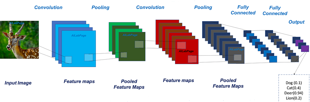 CNN

# Use case 2: CNN-based generic object detector

Deep Learning Framework: Pytorch (opens new window) (An open source machine learning framework that accelerates the path from research prototyping to production deployment). Please follow the installation instructions on the framework's official website (opens new window).

Architecture: The CNN model consists of three convolutional layers and two fully connected layers. Each convolutional layer uses a kernel of size 5 with a stride of 1 and rectified linear units, ReLU, are used as the activation function. After each of the first two convolutional layers, a max-pooling layer of size 2 with a stride of 2 is used. The network was trained over 50 epochs using the stochastic gradient descent (SGD) optimizer. For the first 30 epochs, the learning rate is set to 0.0001 and then it is updated to 0.00001.

The CNN implementation is as follows:

import torch.nn as nn
import torch.nn.functional as f
class cnn_model(nn.Module):

    def __init__(self):

        super(cnn_model, self).__init__()

        self.conv1 = nn.Conv2d(
            in_channels=1,
            out_channels=32,
            kernel_size=5,
            stride=1,
            padding=0
        )

        self.conv2 = nn.Conv2d(
            in_channels=32,
            out_channels=64,
            kernel_size=5,
            stride=1,
            padding=0
        )

        self.conv3 = nn.Conv2d(
            in_channels=64,
            out_channels=128,
            kernel_size=5,
            stride=1,
            padding=0
        )


        self.fc1 = nn.Linear(
            in_features=18*18*128,
            out_features=2046
        )

        self.fc2 = nn.Linear(
            in_features=2046,
            out_features=4
        )

    def forward(self, val):
        val = f.relu(self.conv1(val))
        val = f.max_pool2d(val, kernel_size=2, stride=2)
        val = f.relu(self.conv2(val))
        val = f.max_pool2d(val, kernel_size=2, stride=2)
        val = f.relu(self.conv3(val))
        val = val.view(-1, 18*18*128)
        val = f.dropout(f.relu(self.fc1(val)), p=0.5, training=self.training)
        val = self.fc2(val)

        return val

Source code to learn the model:

import torch
import torch.nn as nn
import torch.optim as optim
from torch.utils.data import DataLoader
import numpy as np
import pandas as pd
from functions import overlapScore


from cnn_model import *
from training_dataset import *

def train_model(net, dataloader, batchSize, lr, momentum):
    criterion = nn.MSELoss()
    optimization = optim.SGD(net.parameters(), lr=lr, momentum=momentum)
    scheduler = optim.lr_scheduler.StepLR(optimization, step_size=30, gamma=0.1)

    for epoch in range(50):

        scheduler.step()

        for i, data in enumerate(dataloader):
            optimization.zero_grad()

            inputs, labels = data

            inputs, labels = inputs.view(batchSize,1, 100, 100), labels.view(batchSize, 4)

            outputs = net(inputs)

            loss = criterion(outputs, labels)
            loss.backward()
            optimization.step()

            pbox = outputs.detach().numpy()
            gbox = labels.detach().numpy()
            score, _ = overlapScore(pbox, gbox)

            print('[epoch %5d, step: %d, loss: %f, Average Score = %f' % (epoch+1, i+1, loss.item(), score/batchSize))

    print('Finish Training')


if __name__ == '__main__':
    # Hyper parameters
    learning_rate = 0.0001
    momentum = 0.9
    batch = 100
    no_of_workers = 2
    shuffle = True


    trainingdataset = training_dataset()
    dataLoader = DataLoader(
        dataset=trainingdataset,
        batch_size=batch,
        shuffle=shuffle,
        num_workers=no_of_workers
    )

    model = cnn_model()
    model.train()

    train_model(model, dataLoader, batch,learning_rate, momentum)
    torch.save(model.state_dict(), './trained_CNN_model.pth')

Source code for handling the dataset (reading data samples):

import numpy as np
import pandas as pd
import torch
from torch.utils.data import Dataset, DataLoader

class training_dataset(Dataset):
    def __init__(self):
      # Training set and corresponding ground truth images
        trainX = np.asarray(pd.read_csv('./my_dataset/trainingData.csv', sep=',', header=None))
        trainY = np.asarray(pd.read_csv('./my_dataset/ground-truth.csv', sep=',', header=None))
        self.features_train = torch.Tensor(trainX)
        self.groundTruth_train = torch.Tensor(trainY)

        self.len = len(trainX)


    def __getitem__(self, item):
        return self.features_train[item], self.groundTruth_train[item]

    def __len__(self):
        return self.len

The following pseudo-code entails a function to calculate the overlap rate taking into account the ground truth boxes and the predicted bounding boxes.

import numpy as np

def overlap(rect1, rect2):

    avgScore = 0
    scores = []

    for i, _ in enumerate(rects1):

        rect1 = rect1[i]
        rect2 = rect2[i]

        left = np.max((rect1[0], rect2[0]))
        right = np.min((rect1[0]+rect1[2], rect2[0]+rect2[2]))

        top = np.max((rect1[1], rect2[1]))
        bottom = np.min((rect1[1]+rect1[3], rect2[1]+rect2[3]))

        # area of intersection
        i = np.max((0, right-left))*np.max((0,bottom-top))

        # combined area of two rectangles
        u = rect1[2]*rect1[3] + rect2[2]*rect2[3] - i

        # return the overlap ratio
        # value is always between 0 and 1
        score = np.clip(i/u, 0, 1)
        avgScore += score
        scores.append(score)

    return avgScore, scores

# Real-time object detection and segmentation with Tensorflow

The objective of this use case is to explain the real-time object detection and segmentation by an example. To do this, we will develop a real-time segmentation application with a simple webcam. We will use the Tensorflow framework (opens new window), the Mask RCNN network learned with the COCO dataset; which allows us to detect up to 100 different types of objects.

First of all, let's make a list of our tools and libraries to install.

Linux Ubuntu
Python
Tensorflow
Open CV

In order to check if your computer is ready, open a python3 console in the terminal by typing python3. Do the following imports:

import cv2
import numpy as np
import tensorflow as tf
from object_detection.utils import label_map_util
from object_detection.utils import ops as utils_ops
from object_detection.utils import visualization_utils as vis_util

To make the model work, you need to load the network and its weights. You will find a list of all object detection models available with Tensorflow on this zoo model. For this tutorial, download mask_rcnn_resnet101_atrous_coco.

We start with the last point: initialize the webcam. This allows two things: (1) to create the video stream and (2) to get the width and height of a frame of the stream in order to configure the output tensor of the mask.

# Init the video stream (with the first plugged webcam)
cap = cv2.VideoCapture(0)
if cap.isOpened():
  # get vcap property
  global_width = int(cap.get(cv2.CAP_PROP_FRAME_WIDTH))
  global_height = int(cap.get(cv2.CAP_PROP_FRAME_HEIGHT))

The next step is to import the label_map file. It is done using methods delivered with Tensorflow's object_detection.

label_map = label_map_util.load_labelmap("PATH/TO/LABELS")
categories = label_map_util.convert_label_map_to_categories(
  label_map, 
  max_num_classes=NUM_CLASSES,
  use_display_name=True)
category_index = label_map_util.create_category_index(categories)

We then proceed with the import of the model and the collection of the tensors.

# Init TF Graph and get all needed tensors
detection_graph = tf.Graph()
with detection_graph.as_default():
  # Init the graph
  od_graph_def = tf.GraphDef()
  with tf.gfile.GFile("/chemin/vers/*.pbb') as fid:
    serialized_graph = fid.read()
    od_graph_def.ParseFromString(serialized_graph)
    tf.import_graph_def(od_graph_def, name='')

  # Get all tensors
  ops = tf.get_default_graph().get_operations()
  all_tensor_names = {output.name for op in ops for output in op.outputs}
  tensor_dict = {}
  for key in ['num_detections', 'detection_boxes', 'detection_scores', 'detection_classes', 'detection_masks']:
    tensor_name = key + ':0'
      if tensor_name in all_tensor_names:
        tensor_dict[key] = tf.get_default_graph().get_tensor_by_name(tensor_name)

  # detection_masks tensor need ops
  detection_boxes = tf.squeeze(tensor_dict['detection_boxes'], [0])
  detection_masks = tf.squeeze(tensor_dict['detection_masks'], [0])
  # Reframe is required to translate mask from box coordinates to image coordinates and fit the image size.
  real_num_detection = tf.cast(tensor_dict['num_detections'][0], tf.int32)
  detection_boxes = tf.slice(detection_boxes, [0, 0], [real_num_detection, -1])
  detection_masks = tf.slice(detection_masks, [0, 0, 0], [real_num_detection, -1, -1])
  detection_masks_reframed =  utils_ops.reframe_box_masks_to_image_masks(
detection_masks, detection_boxes, global_height, global_width)
  detection_masks_reframed = tf.cast(tf.greater(detection_masks_reframed, 0.5), tf.uint8)
  # Follow the convention by adding back the batch dimension
  tensor_dict['detection_masks'] = tf.expand_dims(detection_masks_reframed, 0)

  image_tensor = tf.get_default_graph().get_tensor_by_name('image_tensor:0')

Let's continue our program with the main method. In this method which is called after the initializations we just presented, we capture the last image of the webcam, we process it, we display the modified image and we start again. So the main method works like this:

if __name__ == '__main__':
  # Do that here and save a lot of time
  with detection_graph.as_default():
    with tf.Session(graph=detection_graph) as sess:
      while True:
        # Get the last frame
        frame = cap.read()[1]
        # Process last img
        new_frame = detect_objects(image_np, sess)
        # Display the resulting frame
        cv2.imshow('new_frame', new_frame)
        if cv2.waitKey(1) & 0xFF == ord('q'):
          break

And so the core of the program is in the detect_objects() method which takes as arguments the image (in NumPy array format) and the Tensorflow session which will allow us to run our model.

def detect_objects(image_np, sess):
  # Run inference
  output_dict = sess.run(tensor_dict, feed_dict={image_tensor: np.expand_dims(image_np, 0)})

  # all outputs are float32 numpy arrays, so convert types as appropriate
  output_dict['num_detections'] = int(output_dict['num_detections'][0])
  output_dict['detection_classes'] = output_dict['detection_classes'][0].astype(np.uint8)
  output_dict['detection_boxes'] = output_dict['detection_boxes'][0]
  output_dict['detection_scores'] = output_dict['detection_scores'][0]
  output_dict['detection_masks'] = output_dict['detection_masks'][0]

  # Display boxes and color pixels
  vis_util.visualize_boxes_and_labels_on_image_array(
    image_np,
    output_dict['detection_boxes'],
    output_dict['detection_classes'],
    output_dict['detection_scores'],
    category_index,
    instance_masks=output_dict.get('detection_masks    use_normalized_coordinates=True)

  return image_np

← Object Tracking based on Deep Learning Impactful Presentations →